An Intuitive Understanding of AI Diffusion Models

The classic papers describing diffusion are full of dense mathematical terms and equations.

For many (including myself) who haven’t stretched those particular math muscles since diff eq class a decade or so ago, the paper is just an opaque wall of literal Greek.

In this post I describe my personal understanding of diffusion models in less-dense terms. We will still use some math, but it will be well explained.

Ideally, anyone who has taken algebra should be able to understand this post, yet it should still be useful to AI practitioners.

This post won’t follow a standard treatment of diffusion models. We will deep dive on aspects that I found non-intuitive and skim parts where theory might go deep, but is simpler to understand.

Pre-Reqs

I am assuming basic understanding of the working principles of stochastic gradient descent (SGD) and neural networks in general.

If you are looking for a resource to learn from the ground up, don’t be overwhelmed or discouraged, there are many great videos and tutorials.

My only recommendation is that it’s best to learn by doing: just start training models (RL is a fun place to start).

What is a diffusion model?

basic diffusion process illustration

Diffusion models are their own special class of model because of the particular way that they incrementally “step” towards a solution instead of generating it all at once.

There are different kinds of diffusion models now, like block diffusion and so-called “discrete diffusion” language models.

We are going to focus on diffusion models in the context of generating text-conditioned images.

Originally, models like Stable Diffusion used the UNet as the denoiser backbone.

Newer architectures like the Diffusion Transformer (DiT) serve the same denoising role and follow the same diffusion principles, but use a transformer backbone instead.

The concepts we discuss here are applicable to any diffusion architectures including ones that haven’t been invented yet.

For those who have heard of alternative formulations like rectified flow models: We are only focusing on the diffusion formulation in this post. Many of the concepts extend to rectified flow, but the mathematical formulations differ in some important ways.

What do diffusion models do?

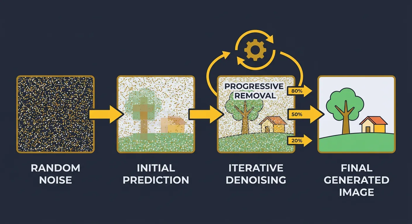
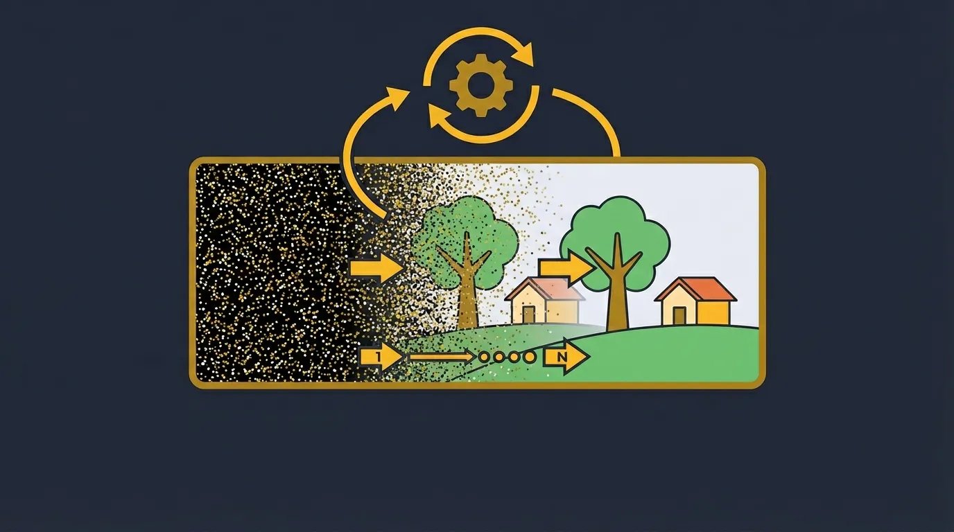
In inference, diffusion models start from pure Gaussian noise and step-by-step turn that noise into an image (or audio, etc…). Non-intuitively this is called the “reverse process”.

What does training look like?

diffusion training process

Training is surprisingly simple: we add noise to a clean image, then train the model with a mathematically convenient proxy for ‘get back the clean image.’

In practice, that proxy is usually $\epsilon$ (the added noise), $v$ (a timestep-dependent combination of image and noise), or even $x_0$ (the clean images themselves).

This is a single MSE loss term!

There are some important details here though:

Diffusion uses fixed timesteps that define the ratio of noise to image.
Typical training uses 1000 timesteps indexed from 0-999.
Early timesteps are mostly image.
Late timesteps are mostly noise.
A schedule controls the amount of noise at intermediate timesteps.
Common schedules include linear and cosine.
We will skip schedule math in this post.
We will focus on the noise-addition rule.

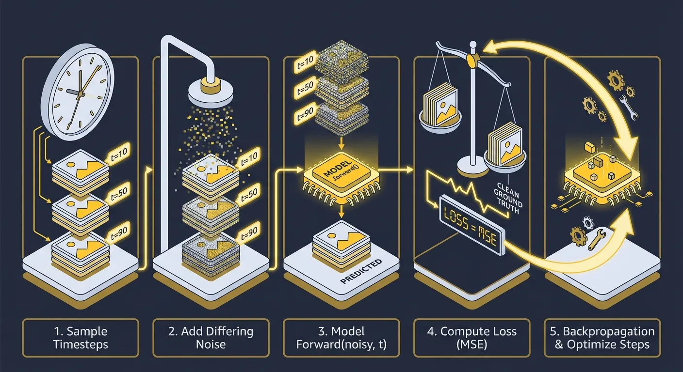
The training loop has these simple steps:

Sample timesteps for every element in the batch.
Add differing noise to each batch element according to those timesteps.
Call the .forward() method of our model, providing both the noisy image and the timestep: model(noisy_images, timesteps)
Compute loss = F.mse_loss(model_output, clean_image_proxy_target)
Do backpropagation and optimizer steps.

Note

Taking a look at the DDPM paper mathematics, this conceptually simple loss function is described like this (equation 14):

L_{\mathrm{simple}}(\theta) \coloneqq \mathbb{E}_{t, x_0, \epsilon}\left[\left\|\epsilon - \epsilon_\theta\left(\sqrt{\bar{\alpha}_t}x_0 \allowbreak + \sqrt{1-\bar{\alpha}_t}\epsilon,\allowbreak t\right)\right\|^2\right]

View explanation

This equation is equivalent to:

timesteps = sample_timesteps()
noise = torch.randn_like(images)
noisy_images = add_noise(images, noise, timesteps)
model_output = model(noisy_images, timesteps)
loss = ((noise - model_output)**2).mean()

Firstly, this model is parameterized to try and predict the noise that was added to the images. This is the $\epsilon$ parameterization.

$\epsilon$ output can easily be converted into the clean output, hence the ‘get back the clean images’ loss proxy.

$L_{\mathrm{simple}}(\theta) \coloneqq$ is loss =
$t$ are the sampled timesteps
$\epsilon$ is noise
$x_0$ are the clean images
$\sqrt{\bar{\alpha}_t}x_0 + \sqrt{1-\bar{\alpha}_t}\epsilon$ are the noisy_images (we examine this noising process below)
$\epsilon_\theta(...)$ is the model() call.
$\left\|\epsilon - \epsilon_\theta\left(...\right)\right\|^2$ is simply squaring the difference between noise and model_output.
$\mathbb{E}$ is the symbol for ‘expectation’ which just means taking the average. Together with the squared difference, this forms the MSE (mean squared error) loss.

For such capable models, the simplicity of the training process is surprising.

There is some masked complexity here though and to understand it we need to dive deep into step 2 (adding noise).

Adding Noise to the Images

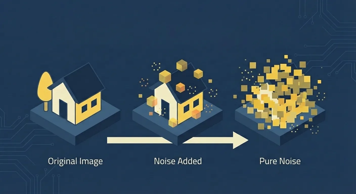
diffusion training adding noise to images

The method used to add noise to images is somewhat non-intuitive.

One might expect a simple linear interpolation: noisy_image = alpha * image + (1-alpha) * noise

Or perhaps simply adding noise like sampling (the Variance-Exploding (VE) setup): noisy_image = image + alpha * noise

But diffusion models use a special type of noise addition called “variance preserving” noise addition: noisy_image = sqrt(alpha) * image + sqrt(1-alpha) * noise

If you are studying the papers and different implementations it gets even more confusing as sometimes you will see this formulation:

$x_t = \sqrt{\bar{\alpha}_t}\,x_0 + \sqrt{1-\bar{\alpha}_t}\,\epsilon$

$x_t$ here is the noised image where t stands for timestep, $x_0$ is the clean image, and $\epsilon$ is the sampled noise.

Or this equivalent one:

$x_t = \sqrt{\alpha}\,x_0 + \sqrt{1-\alpha}\,\epsilon$

And sometimes you will see this one:

$x_t = \alpha_t x_0 + \sigma_t \epsilon$

Paired with something like this:

$\alpha_t^2 + \sigma_t^2 = 1$

These are all ways of writing the same thing; in the third form, $\alpha_t$ and $\sigma_t$ already absorb the square roots.

This is important because $\alpha$ and $\bar{\alpha}_t$ are not universal terms amongst papers and especially amongst implementations. It changes the way other equations and the alpha schedule (according to timestep) gets interpreted.

In the first formulation, timesteps map to $\bar{\alpha}_t \in [0,1]$ (which just means it is in the range 0 to 1, inclusive). In the third, the same timestep is written with a pair $(\alpha_t, \sigma_t)$ .

Anyways, armed with this knowledge, we can better understand papers and implementations that we study.

What is Variance Preserving Noise

Loading simulation...

The interactive simulation above gives a visual intuition for what variance-preserving (VP) noise is doing compared to linear interpolation.

Look at the bottom graph first: in VP noise, alpha + sigma is usually not 1, which can appear to create a strange scaling of the noisy image at first glance.

Now look at the graph above it: the signal energy stays essentially flat in the VP formulation. So even though alpha and sigma do not add to 1, the overall scale of the noised signal stays stable.

How does Variance Preserving noise Preserve Magnitude?

This behavior was deeply non-intuitive to me at first. Why doesn’t linear interpolation preserve magnitude?

Linear interpolation says: “take some percentage of the image and some percentage of noise.” If those weights sum to 1, that feels balanced in the everyday sense. But that only preserves magnitude if both vectors point in the same direction, which they do not.

Image and noise mostly act like different directions, so their sizes do not combine like plain numbers.

A useful intuition is moving right and up:

going 1 unit right and 1 unit up does not put you 2 units from where you started
it puts you $\sqrt{2}$ units away

That is the same kind of combination happening here. The image contributes in one “direction” and the noise contributes in another. To keep overall magnitude steady, you do not want coefficients that merely add to 1. You want squared contributions that add to a constant.

So the key is: we are not preserving a blend ratio, we are preserving average energy.

That is why VP noise can keep magnitude stable even when alpha + sigma != 1.

Another Intuitive Approach to Noise Mixing

The motivation for VP noise can be viewed as one “intensity budget” split between image and noise.

Early timesteps allocate most of that budget to the image. Later timesteps allocate most of it to noise. VP keeps the total budget roughly constant, so we are redistributing intensity rather than accidentally making everything dimmer or brighter over time.

An intuitive contrast with linear interpolation is a crossfade between a clean photo and pure static. With linear interpolation, the midpoint is 50/50 by coefficient, but not 50/50 by energy.

Because image and noise are largely independent, their contributions combine through squares, not plain addition. With linear interpolation total energy dips in the middle and the mixture looks washed out.

You can actually observe this effect by slowly sliding the slider from the left to the right in the above simulation. The linearly interpolated image colors appear to get a slight film over them.

Diffusion Models at Inference Time

diffusion noise to image

Now that we understand the motivations behind the noise addition process, let’s move onto the complexities of using diffusion models to actually generate things.

When we naively try to use diffusion models to actually generate images, we quickly run into issues. A single step of the model from pure noise produces garbage.

Newer methods like DMD and Consistency Models can achieve single step generation, but we are talking about vanilla diffusion here.

We explicitly trained the model with an MSE loss against a proxy for clean-image recovery, so why would it be malfunctioning on us when we actually try to use it?

To understand this, we are going to first examine the MSE loss.

MSE Loss

Loading MSE simulation...

Simply put: given an input that can map to two points with equal probability, the optimal loss value for MSE loss is in the average of these points (conceptually: in the middle of the points).

For diffusion models, when it sees pure noise, this can map to many, many different images, so the model learns to output the average of all these probable mappings, rather than a single, clean image.

You might be thinking, “no, I told the model to make a cat image”, but unless you described the complex matrices of position and deformation for every single strand of hair on that cat (not to mention other details), there is still going to be variation that gets averaged against.

Progressive Self-Generated Conditioning

You might be asking yourself, “if the model only learns averages, how do we get any decent images output at all then?”

I have formed my own intuition for this that I call “progressive self-generated conditioning”.

This is not a standard terminology or method of describing this process, but I have found it to be a useful and effective intuitive framework.

With an mse loss, a model learns to map to average potential points, but there is another input called conditioning. In text-to-image models, this conditioning takes the form of text (the prompt).

Conceptually: the conditioning constrains the possibilities that the noise can be interpreted into, and thereby reduces the range of averages the model maps against. If the text is “a dog” all “cat” endpoint probabilities go to zero.

If we were able to describe every detail of a target image, then the model should theoretically be able to generate that image in one-step, since there is only one possibility, we don’t have to worry about the mse averaging problem.

Extend that concept out from text to the general idea of conditioning, and we can understand how the model overcomes the mse averaging problem during inference.

At each step:

input current noisy image to the model
the model predicts an output averaging all probability-weighted possibilities constrained by the current conditioning (technically this is usually through a proxy like $\epsilon$ or $v$ )
the inference process takes a small step in that direction, reducing noise in the image
repeat until finished

Understand that the noisy image is effectively another form of conditioning.

As the noise reduces, the range of possibilities for the next model invocation iteratively narrows, overcoming the averaging problem a little bit at a time. Hence, “Progressive Self-Generated Conditioning”.

In the DDPM paper, this progressive step is written as $p_\theta(x_{t-1} \mid x_t)$ , which means the possibilities for the next less-noisy image $x_{t-1}$ are conditioned on the current noisy image $x_t$ .

All this in mind, it is easy to see why diffusion models must do inference step-by-step.

In practice, models are frequently post-trained with inherent biases which form implicit conditioning. This process has tradeoffs but is usually a net win for output quality.

Samplers

Loading sampler simulation...

The role of the sampler is simple: convert the model’s output into a step that reduces the noise in our current image estimate.

In math terms: The sampler decides how to turn $x_t$ into $x_{t-1}$ (remember t goes from 999 [pure noise] to 0 [no noise]).

A few things are happening here:

During inference, we usually run far fewer timesteps (around 20-50) than we use during training (typically 1000).
We keep the training timestep schedule and map each inference step onto it (for example, inference step 20 maps to training step 999, 19 to 949, and so on).
The sampler moves from one inference step to the next (18 -> 17, then 17 -> 16), while mapping each move to the corresponding target noise level (alpha and sigma) from the training schedule.
This creates a speed/quality tradeoff: fewer inference steps are much faster, but pushing too low can hurt detail, stability, and fidelity.
Step spacing also matters: how you choose and distribute those 20-50 inference steps across the 1000 training steps (linear, non-linear, etc.) can significantly affect final quality.

There are different types of samplers:

Ancestral (stochastic) samplers: DDPM, Score SDE predictor-corrector.
Implicit/deterministic samplers: DDIM.
Higher-order ODE/SDE solver samplers: PNDM, DPM-Solver, DPM-Solver++.

Samplers are somewhat of a deep topic, and while useful to understand in their own right, we won’t be diving deep into them in this post.

Key Takeaways

Diffusion training is conceptually simple: add noise at a chosen timestep and train on a proxy target (x0, epsilon, or v) for clean-image recovery.
Variance-preserving noise keeps overall signal energy stable as we trade off image content and noise across timesteps.
A one-shot jump from pure noise is hard because MSE pushes the model toward averages over many plausible outputs.
Step-by-step inference works because each denoising step narrows possibilities and provides better conditioning for the next step.
The sampler is the mechanism that converts model output into the next less-noisy state.
Inference usually uses far fewer steps than training, so sampler choice and step spacing directly control the speed vs quality tradeoff.

Where to Go Next

Read the original DDPM paper and then DDIM to connect this intuition to the standard formulations.
Study a known-good minimal implementation: minDiffusion. It is compact and easy to trace step-by-step.
Further research: Variational AutoEncoders, Latent Diffusion, and Classifier Free Guidance.